TLDR: Topological Data Analysis uses abstract maths to uncover hard to spot patterns in high dimensional data. Read more to get an intro with all the complex maths simply explained.

In 2018 coming to the end of my degree I was excited to read that the abstract area of my masters thesis in mathematics had an application in data science: Topological Data Analysis.

What is Topological Data Analysis (TDA) and why do I care? TDA aims to apply mathematical techniques from the intersection of algebra and topology to find shapes and patterns in data that we otherwise would not be able to see. It has been applied over the last decade in areas such as medicine and physics to identify patterns previously missed, such as a subgroup of breast cancers.

The Maths

Let’s start with the area of maths thats used in Topological Data Analysis: algebraic topology. The overall concept we are aiming to get a basic grasp of is that of the ‘Homology groups of a space’.

The Group Theory

The first object we need to get to know is the group. Very roughly a group is a collection of elements which confirm to a certain set of properties and can be combined using certain rules. The best example is the integers, denoted \(\Z = \{\dots,-2,-1,0,1,2\dots\}\).

(The Integers, credit: wikipedia)

This set of numbers forms a ‘group’ under addition, as you can add two integers and get another integer, you can subtract two integers and get another integer and you have the special element \(0\) where for any integer \(x\) if you compute \(x + (-x)\) you get \(0\). For the purpose of this post we don’t need much more, for now just think of a group as a structure which allows an abstract framework to fall into place nicely around it!

The Topology

The next piece we need to tackle is topology. In topology we think of most spaces as very flexible, we can push and pull surfaces around like big sheets of rubber. This is sensible because the properties topologists care about are not changed by these transformations. Given we can do this, topologists then start to care about which spaces are ‘the same’, in that if we take two spaces and we stretch and pull one around can we end up stretching and pulling so much that our first space looks like the second. If so then we call these spaces the same (in maths we would call them homotopic). For example a circle and and oval are homotopic. One to think about a bit more is that the surface of a donut and the surface of a cup are homotopic.

(A mug morphing into a torus, credit: wikipedia)

The surface of a donut, and a football are somehow fundamentally different however, as the donut has that hole through the middle and the ball does not. They are both hollow inside but that hole through the middle of the torus is enough to make the objects fundamentally different in the world of topology.

The One Where The Group Theory And The Topology Met

Enter algebraic topology: Some while ago mathematicians had the bright idea that we can take all of the fancy mathematics that we have developed to study the theory of groups, and try and apply it to study the theory of spaces. Maybe if we can tell groups apart easily, then we can use them to tell spaces apart easily too, as long as we have a nice way of associating groups to spaces?!

This turned out to be a great idea, and they came up with the following process. Take a space and assign to it a series of groups called the homology groups of the space. Let’s number these, so we have the \(m\)-th homology group of a space \(X\) which we denote by \(H_m(X)\). This group tells us about the \(m\)-dimensional holes in our space \(X\). For example a circle (this is just the outline remember, not a solid disk!) has a hole in the middle we will call a ‘\(1\)-dimensional hole’. A (hollow) sphere, aka a football, has a \(2\)-dimensional hole in the middle of it enclosing some volume, and so on. A torus, aka a hollow donut, encloses the same kind of space as a sphere does, but if you can also have loops going around the torus in two directions which can never close, so the torus has two \(1\)-dimensional holes as well.

Let’s now turn the above intuition into maths notation. In each dimension we use a copy of \(\Z\) to represent the presence of a hole, so \(\Z\) means one hole, and \(\Z^2\) means two holes etc. For the sake of this post don’t worry about why this is (for those that know group theory, what we really have is isomorphisms between the integers and the homology groups). Let’s use our new notation to represent the homology groups of the spaces we discussed. (Note: the \(0\)-homology represents how many chunks our space is divided into, one circle will have one lot of \(0\)-homology, two circles separate will have two lots of \(0\)-homology)

For a circle which we denote \(S^1\):

• \(H_0(s^1) = \Z\), (we have one piece of data, the circle in our space)
• \(H_1(S^1) = \Z\), (this is the one hole in a circle)
• \(H_n(S^1) = 0\) for all \(n > 1\).

For a sphere which we denote \(S^2\):

• \(H_0(S^2) = \Z\), (we have one piece of data, the sphere in our space)
• \(H_1(S^2) = 0\), (the sphere does not have the same 1D hole as a cirlce)
• \(H_2(S^2) = \Z\), (the sphere has a ‘hole’ but this time it contains volume so its one dimension up)
• \(H_n(S^2) = 0\) for all \(n > 2\).

For a torus, which we denote \(T\):

• \(H_0(T) = \Z\), (we have one piece of data, the torus in our space)
• \(H_1(T) = \Z^2\), (the torus has a ring going both ways around it, so two lots of the 1D homology a circle has)
• \(H_2(T) = \Z\), (the torus also encloses volume like a sphere, so has 2D homology)
• \(H_n(T) = 0\) for all \(n > 2\).

I understand a lot of the notation is seemingly random but I promise it isn’t, there just isn’t much point going into enough undergrad maths courses to explain it all. The important concept to grasp is that the \(m\)th homology group of a space tells us about the number of \(m\)-dimensional holes in that space.

The Data Science

Now we turn our attention to some data. Given any dataset, what we have are a load of points scattered in space. In order to apply the above techniques we need to make these somehow more ‘solid’, enter the Vietoris-Rips complex! What we do is pick a radius \(\epsilon\) and look around each point within that radius, if there are other points within that radius we join them up. Applying this accross our data set gives us a space we denote \(R_\epsilon\). For each \(\epsilon\) we can create a sequence of Homology groups \(H_1(R_\epsilon), H_2(R_\epsilon), \dots\).

(A Vietoris-Rips complex, credit: wikipedia)

As \(\epsilon\) increases in size different features become apparent in our complex, and so parts of the homology may appear at one \(\epsilon_1\) and dissapear at some other \(\epsilon_2\). For example consider a data set of a circle of points. When \(\epsilon\) is small the space we form is a circle, however at some point \(\epsilon\) will get so big that all of the points join into one to make a disk. Hence we see the \(H_1\) changes as epsilon increases, the \(\epsilon_1\) where a feature first appears is called the ‘birth’ of that feature, and the \(\epsilon_2\) where a feature dissapears is called the ‘death’ of that feature. We collect all of these pairs of birth and death values together into a set and display them on a diagram called a ‘persistence diagram’.

(Persistence diagram, credit: wikipedia)

To read this diagram, take a point \((\epsilon_1, \epsilon_2)\). The \(x\)-coordinate denotes the birth time of that feature, and the \(y\)-coordinate denotes the death time.

Putting It Into Practice

So now we understand what Topological Data Analysis entails, how can we turn this into actual code to apply to data?! It turns out some very nice people have put together a set of packages in python to compute the Persistent Homology and Persistence Diagrams of a dataset: the scikit-tda python package. Just run ‘pip3 install scikit-tda’ (note you may need cython as a prerequisite).

For starters you can use ripser to compute your homology and persim to plot your persistence diagrams from this data. Let’s take a simple example to demonstrate what we have learned here. Using sklearn we generate a dataset of two circles of points very close together.

from sklearn import datasets
import matplotlib.pyplot as plt
from ripser import ripser
from persim import plot_diagram
import numpy as np
data = datasets.make_circles(n_samples=80, factor=0.99)[0]
plt.scatter(data[:,0], data[:,1])

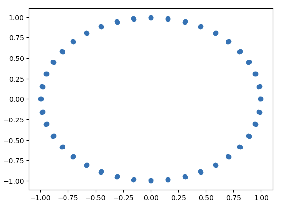
Let’s now use persim to plot the persistence diagram from this data.

diagrams = ripser(data)['dgms']
plot_diagrams(diagrams, show=True)

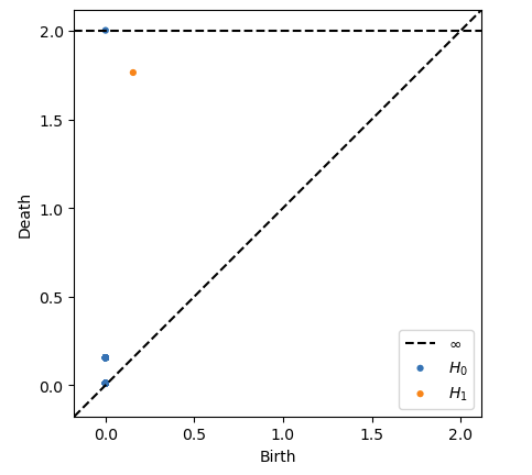
We see a very persistant feature in the \(1\)-homology relating to the hole inside the circles, and a persistent point in the \(0\)-homology relating to the fact we have roughly one overall cluster of points.

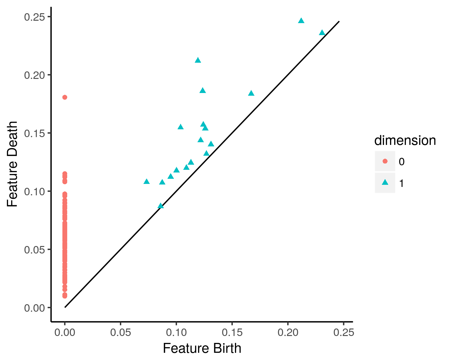
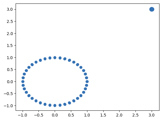
Let’s now create a tiny circle off to the right of our main circle.

extra_circle_data = np.concatenate([datasets.make_circles(n_samples=80, factor=0.99)[0],
              3+0.03*datasets.make_circles(n_samples=80, factor=0.99)[0]])
plt.scatter(extra_circle_data[:,0], extra_circle_data[:,1])

We can use the above code to create the following persistence diagram from the new data.

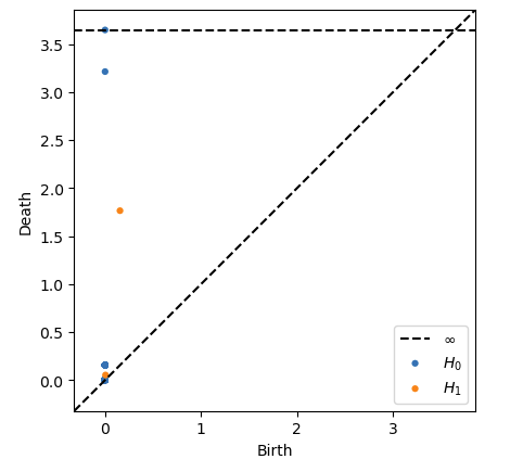
Note now the extra elements of \(0\)-homology which we can relate to the new point clustering, and the very small new piece of \(1\)-homology which we can relate to the tiny new hole inside our very small circle. You can see how the topological features of the data have been captured here.

For more nice graphics of data and persistence diagrams checkout this blog.

Next Steps

Now you have seen some Topological Data Analysis in action, take your favourite dataset and run it through the libraries from scikit-tda, to see what patterns may be revealed. The above is really just the bare minimum you need from mathematics to understand some of the concepts here, there is lots I glossed over for simplicity and the interested reader has many tens of hours of abstract algebra, point set topology and homological algebra to read before the standard algebraic topology makes sense from the ground up. However in order to just apply TDA in practice much less of this is needed, and hopefully this post has been able to demistify some of that high barrier to entry.

If readers are interested in further exposition on TDA, or more on the mathematics behind TDA I am happy to write further posts, just shoot me a message (linkedIn is easiest)!

Advanced Topics and Further Reading

Further group theory: Warwick’s Introduction To Abstract Algebra

Further algebraic topology: Hatcher’s Algebraic Topology (note: this is the free copy published by Alan Hatcher himself)

Introduction to TDA (much more in depth than here): Murugan et al, Arxiv Paper

Example of an application of topological data analysis: Gidea et al, Arxiv Paper